CSMODEL_midterm_exam_megadoc
This note has not been edited yet. Content may be subject to change.
EDIT (10/08/2025 6:48PM): copy pasted the contents sana gumana
EDIT (10/08/2025 7:36PM): removed the TOC, please use the one on the right! thank you + vercel is rate limited pls refer to the render site <3
also i'm aware of the latex not rendering properly so sorry. pls dm me @clavzno on discord for a pdf
EDIT (10/09/2025): fixed the problem with latex
1a Introduction to Data 🟢
Examples of Data
Types of Data
Forms of Data
Data Modelling
Data Collection and Sampling
- Data refers to pieces of facts and statistics collected and recorded for the purposes of analysis
- Dataset: a collection of related pieces of data
Types of Data
- Categorical (descriptive information, may have several categories)
- Ordinal (have a sense of ordering)
- Nominal (no order)
- Numerical (can objectively be measured)
- Discrete (specific value)
- Continuous (can take any value within a range)
Forms of Data
- Structured: adheres to some structured model
- Unstructured: does not adhere to a standardized format
- Graph-based: represented as pairwise relationships between objects
- Natural Language: information expressed in human language
- Audio & Video: not represented in text format
- Generated: recorded by applications without human intervention
Data Collection
Collected by other people
- Public online sources: data made public over the internet
- Private sources: contacting people or organizations to request for data
Collected by you - Observational Study: data where no treatment has been explicitly applied
- researchers perform an observational study when they collect data in a way that does not interfere with how the data arise
- Experiment: data collected from studied where treatments are assigned to cases
- researchers perform an experiment by applying treatment to an experimental group and comparing it against an untreated control group.
Correlation ≠ Causation
In an observational study, only correlation, or relationship between variables can be concluded.
An experiment is needed for causation to be established, by isolating all other variables aside from the one being treated
More on Data Collection
Data may be collected not for any specific research question or purpose, by just collected for future potential analysis
Data could already exist somewhere in the world, waiting to be collected for some research goal or purpose
Sampling
- Population: the entire group of elements to which you intend to generalize your data on → in the real world, it's not possible
- A sample is collected to represent the entire population → if collected properly it can be generalized to the entire population.
- The sample should be chosen randomly to avoid bias, where the sample is skewed towards certain groups and does not represent the whole group
Sampling Bias
- Convenience Bias - Only the data that is easy to collect is included in the sample.
- Nonresponse Bias - Some chosen participants are unwilling to give data.
- Voluntary Response Bias - Only people who are willing to volunteer are included in the sample.
- Exclusion Bias - some groups are deliberately excluded to participate in the data collection.
Simple Random Sampling
- randomly select observations from the population
Stratified Random Sampling
SimplePsychology: Stratified Sampling
- arrange the population according to some meaningful groupings or strata
- members in a stratum are homogeneous and members of a stratum are heterogeneous from member of another stratum
- randomly sample from each group to get the desired number of sample (ex. get 3 from each of the 4 groups to get a total sample size of 12)
Cluster Sampling
- divide the population into natural groups (address, age, sex, etc.)
- further grouped according to their address
- choose clusters to include the sample
Multistage Sampling
- extends cluster sampling
- Stage 1: select clusters to be included in the sample
- Stage 2: randomly sample from the selected clusters
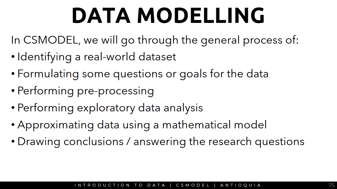
Data Modelling
- preprocessing steps must be performed to make use of the data
- the process is motivated by an overarching research question or goal
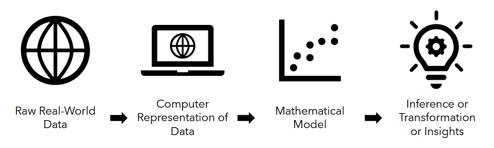
- get the raw data
- load the data into a format understandable by computers
- estimate or represent the data using a systematic mathematical model
- then make conclusions, transformations, or generate insights from the model
Modelling should be backed-up by a research question
- should be clear and concise (easy to understand, easy to explain to others, free of technical jargon)
- feasible (could be answered using the available data and resources at your disposal)
- meaningful (addresses a real problem, not something trivial or obvious)
Answering the research goal or question
- Data preprocessing
- Exploratory Data Analysis
- Data Modelling
1. Data Preprocessing
real world data is dirty
- incomplete - missing values
- noisy - may contain outliers or errors in measurement
- inconsistent - may contain discrepancies in encoding
if the data is analyzed without preprocessing it may result in low-quality results - preprocessing steps are often done to clean the data of these problems
- other data preprocessing techniques may also be done, like discretization or normalization, depending on the data
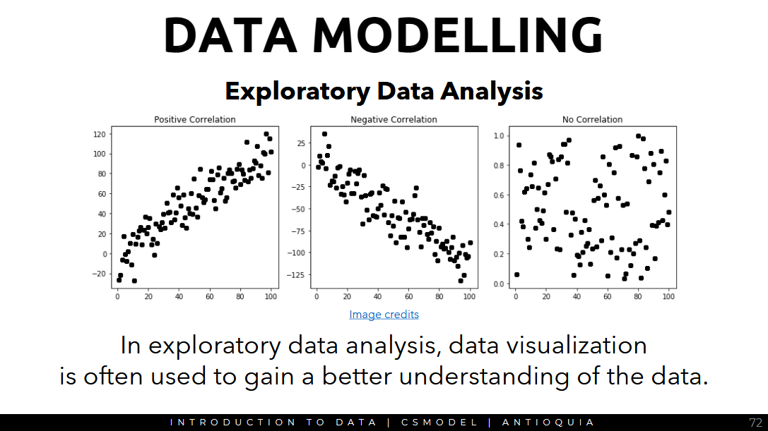
2. Exploratory Data Analysis
lets you build a general understanding of
- the relationship between different variables
- distribution of the different variables
- outliers in the data, if any
- general characteristics of the data as a whole
performing exploratory data analysis can sometimes help identify good research questions
data visualization is used to gain a better understanding of the data
Mathematical Models
- data modelling involves creating a mathematical approximation of the data
- mathematical model: represents the data in a systematic way, where mathematical techniques can be applied to make comparisons, transformations, and conclusions
mathematical models allow us to
- describe/summarize the data systematically
- make comparisons systematically
- make inferences supported with statistical confidence
- statistical inference: means drawing conclusions in the presence of uncertainty
1b Data Representation 🟢
Dataframe and Series
Basic Operations
Python Crash Course
Data must be represented into a data structure to apply computer algorithms for analysis.
Data Matrix
- literally just a table
- each row is a single observation or instance in the dataset
- each column is a variable, which represents a characteristic of each observation
- each variable has a certain type of data or datatype
Pandas (panel data)
- Python package designed for analysis of tabular data represented as vectors and matrices
- pandas works seamlessly with other data science libraries for python
numpy- optimized basic math operationsmatplotlib- data visualizationscipy.org- advanced math functionsscikitlearn- machine learning
DataFrame
- the primary
pandasdata structure - 2d, size-mutable, potentially heterogeneous tabular data
- size-mutable: you can change its dimensions (number of rows and columns) after it has been created
- the data structure contains labeled axes
- arithmetic operations align on both row and column labels
- kind of like a
dict-like container forSeriesobjects
Series
- 1d ndarray with axis labels
- labels don't need to be unique
- the object supports both integer- and label-based indexing
- operations between
Seriesalign values based on their associated index values - they do not need to be of the same length
More on DataFrame
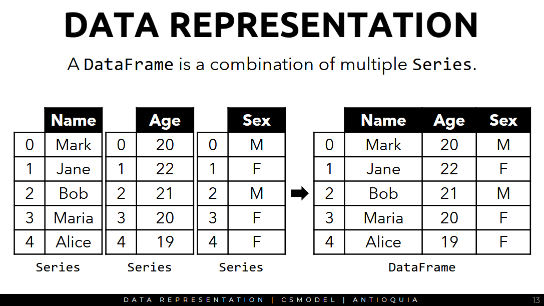
-
a
DataFrameis a combination of multipleSeriesobjects
-
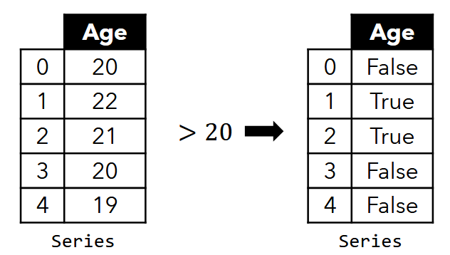
applying on operation on a Series by a scalar performs the operation on each member of the Series
-
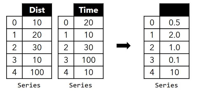
applying an operation on a Series and another Series performs the operation element-wise
-
You can use
?in Jupyter for any function to quickly view its documentation
import pandas as pd
?pd.read_csv # read_csv is a function
Basic Operations
- View dataset info - view dataset information such as variables, datatype of each variable, number of observations, the number of missing values, etc.
- Select columns - select one column as a
Seriesor select 2 or more columns as aDataFrame - Select rows - select a single observation as a
Series, select 2 or more observations as aDataFrame - Filter rows - uses a conditional (like select observations where CSMODEL grade ≥ 3.0)
- Sort rows - ascending or descending
- Add new columns - add a new column to the DataFrame where (condition) (ex. Add a new column "Type" where the value is Good if CSMODEL grade ≥ 3.0 and "Okay" otherwise)
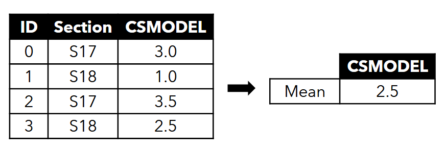
- Aggregate Data - get the average (or mean, median, etc.) of a column
- "aggregate": combining or summarizing multiple individual data points into a single, higher-level value or a smaller set of values. (common functions include ∑, average/mean, count, min, max, median, mode)
- "aggregate": combining or summarizing multiple individual data points into a single, higher-level value or a smaller set of values. (common functions include ∑, average/mean, count, min, max, median, mode)
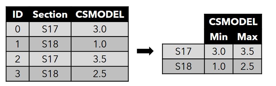
- Group by variable - Group the data by section then get the min and max grade per section for CSMODEL
2a Data Preprocessing 🟢
Data Cleaning
Pre-processing Techniques
Data Cleaning
- raw data in the real world, is inherently dirty
- in data cleaning, these inconsistencies are addressed to prevent problems in analysis
- "in data science, 80% of time spent to prepare data, 20% of time spent to complain about need to prepare data"
Separate Files
- data comes from multiple sources, collected at different times, and/or completely different datasets
- use various pandas functions such as
concat()andmerge()to combine separate files
Multiple Representations
- different representations of text may occur in the dataset
- use the
unique()function to ensure that categorical variables are correctly represented - you can also use the
map()function if you want to modify the values by assigning the same value for each categorical level
Incorrect Datatypes
- numerical values in the dataset may be represented as text or string
- use the
info()function to check the datatype of each column in the dataset - can be used to convert all variables to appropriate numerical datatype.
- use the
apply()function the appropriate column and use a lambda function to convert each element into a numerical data type
Default Values
- datasets may use a default value for when the data is missing or not applicable
- handle these cases appropriately depending on the context
- in pandas, missing values are represented as
NaNorNone. Make sure they're represented as that.
For other kinds of default values, handle them based on context.
Missing Data
- elements in the dataset may be missing because the data is unavailable
- handling missing data depends on the domain or the context. use your own judgement.
- option: delete all rows that contain missing data
- option: replace the missing data with the mean of the variable, and so on
Duplicate Data
- a dataset may contain duplicate data
- in some cases there really is a duplicate, other cases it may be an error.
- in pandas you can use
drop_duplicates()to delete duplicates in the dataset
Inconsistent Format
- date and time may be recorded in inconsistent formats due to human error, inconsistencies in data collection and encoding, or different locale and formats
Data Preprocessing
Querying
- use the
query()function ofpandasto write complex conditions for selecting appropriate info from the dataset - the
query()function queries the columns of aDataFramewith a Boolean expression - provides a more streamlined syntax for getting a subset of the
DataFrame
df = pd.DataFrame({
	"ID": [0, 1, 2 ,3, 4],
	"CCPROG1", [3.0, 1.0, 3.5, 2.5, 4.0],
	"CCPROG2: [1.0, None, 4.0, 1.0, 4.0]
})

df.query("CCPROG1 >= 3.5") # give it a Boolean value
# we should be able to have row 2 and 4 selected
df.query('SECTION == "S17"') # query based on String value
# query rows based on multiple conditions
df.query("CCPROG1 >= 3.5 and Section == 'S17'")
df.query('index > 2') # returns rows 3 and 4, index is a reserved keyword
df.query('CCPROG1 > CCPROG2') # you would get index 0 and 3 (you cant compare a numerical value and none value)
Note: None is not necessarily 0
Looping
- user
iterrows()to iterate over all rows and apply some operation to each row cur_idxis the index of the current row andcur_rowis the actual rowcur_rowshows each row data
for cur_idx, cur_row in df.iterrows():
	# perform some operations
- previously we used
iloc()but there's multiple ways of doing it
Inplace parameter
- some pandas functions, there's an option called inplace
- by default it's set to
inplace=false - for example,
drop_duplicates()will not affect the original df but will only show you the selection. - if you want to use the original df, specify
inplace=True. it will change the originaldataframeobject
Imputation
- datasets with missing values can be a result of error in the data collection process, privacy/refusal to give information, or interruptions/failure in sensors
- rows with missing values might be dropped from the dataset, but it might not be the best approach in all cases.
Method 1
- use a threshold value
tto decide whether to drop or not - drop columns with missing value less than the threshold t:
df = df[df.columns[df.isnull().mean() < t]] - drop rows with missing values less than the threshold t:
df = df.loc[df.isnull().mean(axis=1) < t]] - what's the best threshold value? it's on a case-by-case basis (sir couldn't give a best threshold value)
- personal rule of thumb, if it's 90% null, he'll drop it
- for columns with no null values, you could do a separate sub-analysis for that particular population
Method 2
- another approach is imputation, where missing values are estimated based on existing values
- numerical imputation
- categorical imputation
Numerical Imputation
- use the median/mean or average of the other values as an estimate of the missing values
- NOTE: check the dataset to see whether this is a good idea or not
- ex. age of one person is missing, use the median age of all the other people in the dataset to estimate the age of that person - the missing age is likely the same as the most common age in the dataset <- justification is statistically likely
Categorical Imputation
- use the mode as the estimate for the missing values
- NOTE: this might not be the best approach if theres no dominant value in the dataset, and the values are approximately uniformly distributed
- ex. a person's smoking information is missing. however 95% of the people in the dataset are non-smokers. assume the missing value is "non-smoker"
Binning
- technique where data is grouped together into a series of categories
- numerical or categorical
- could reveal relationships and insights in a clearer way that could not easily be seen if the original values were used
- in ML, binning helps overfitting, where models are tailor-fitted to specific examples instead of being able to recognize general cases -> it learns too much that it fails to generalize in a larger, broader concept (CSMODEL doesn't deal heavily with ML)
Numerical Binning
- numerical data is grouped in different ranges of values
- 14 -> 13-15
- 11 -> 10-12
- 10 -> 10-12
- 8 -> 7-9
- 4 -> 4-6
- transforming continuous data into discrete data
Categorical Binning
- for categorical data, they're grouped by related values aka larger subgroups
- malate -> Aanila
- cubao -> QC
- Ermita -> Manila
- BGC -> Taguig
- Quiapo -> Manila
- aggregating, grouping them to make them more general and less granular
- useful in the cases that the dataset is too specific
Outlier Detection
-
outliers are extreme values in the dataset
-
can be detected using different approaches: visualization techniques like scatterplots and line graphs, standard deviation/Z-score, percentiles
- visualization techniques: plotting the data points in a graph; most of the data were clumped together on the lower left and there were outliers on the upper right. the blue line is a linear function. if we fit a linear formula to represent everyone, it's not the best fit but removing outliers made it more accurate
-
use a more quantitative approach by measuring the z-score, or the number of standard deviations from the mean of each data point
-
if our data is nearly normal, then anything outside 3 standard deviations from the mean is an outlier
- get the middle x percent of the data. anything outside the middle x percent is an outlier. we assume most of the data lies within the bell curve. 95% of the data is within that interval, 99.7% should be within 3 standard deviations from the mean value (center value)
-
anything beyond 3 standard deviations is considered an outlier
-
drop: remove the rows with outliers to exclude them from analysis since these might be extreme cases that do not happen normally
-
use a cap: instead of reducing data size, simply clamp the values within the desired range. this can help prevent adverse effects on algorithms and models that are sensitive to outliers but may affect the actual distribution of the data (force everyone to have the same range of values)
- capping isn't normalization, not necessarily. normalization is one form of capping, other times you just forcefully change the values of the extremes
consideration:
- there are many causes of outliers, from errors in encoding to real rare occurrences in the dataset
- by removing or disregarding them, some important insights might be removed from our data
- thus be careful in handling outliers
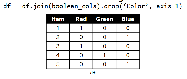
One-hot Encoding
- some data modelling techniques including ML algorithms, require different data representation
- in the Boolean representation, each property is represented as a column where the value is 1 if true and 0 otherwise
- ex. in content-based recommender systems, the item profile was represented as a Boolean vector
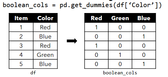
- then you can combine them into one
Log Transformation
-
the log operation
log(n)evaluates to x, where 10^x = n -
NOTE: the relationship between n and log(n) (Big O)
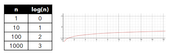
-
by applying the log function to every data point, the values are transformed by reducing the effect of extremely high values while preserving the order
-
log transformations are useful for normalizing skewed data and reducing the impact of outliers but distort the scale of the distance.
-
NOTE: the order of the data points are preserved in log transformation, but the scale of the distances between each datapoint might be distorted
-
GEMINI: the "distortion" of scale is a trade-off. You give up the direct additive interpretability of the original scale to gain benefits like normality, reduced outlier impact, and stabilized variance, which can be crucial for valid statistical analysis and model building. When interpreting results from log-transformed data, it's essential to remember that the effects are often multiplicative on the original scale.
Aggregation
- used to summarize data
- generally performed when we have several rows that belong to the same group or instance
- numerical or categorical
Numerical Aggregation
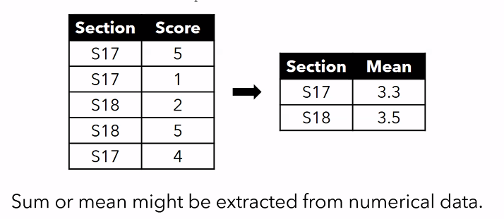
- group df by section, and get the mean score per section
Categorical Aggregation
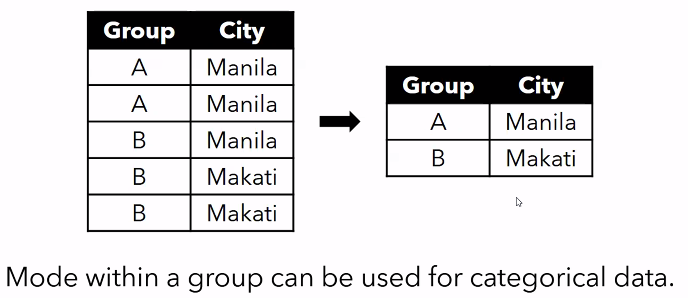
- we want to group A and B by the most frequently occurring data value for city
df_ncr = pd.DataFrame({
	"Group": ["A", "A", "B", "B", "B"]
	"City": ["Manila", "Manila", "Manila", "Makati", "Makati"]
})
df_ncr.groupby(by="Group").agg(pd.Series.mode)
df_cdr['City'].mode() # get the mode of the entire series
Column Transformation
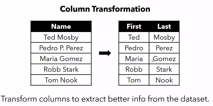
-
if the string contains the full name, you might want to separate it into two separate columns
-
use
apply()function inpandasand then use a custom function to split the string (like separate the name by space, the last set of strings is the first name, etc.) -
transform the dates into better representations since computers cannot understand order given dates like "2019-06-04"
- extract the month, day, and year, and put them in separate columns as numerical values
- use a single numerical representation for each data (e.g. the number of seconds since a constant dates)
-
most computers use ISO standard format
Feature Scaling
- different variables have different ranges
- some algorithms will be affected if one variable "overpowers" others
- ex. Euclidean distance will be affected if the scale of the variables are not equal
Example
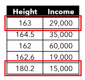
- height is in centimeters
- income is in the thousands range
1. Normalization (min-max normalization)
- scales all the features into a range of 0 to 1
- but susceptible to outliers because the extreme values define the range
2. Standardization (z-score)
- x minus mean over standard deviation
- measures the distance of each point from the mean
- less susceptible to outliers, since it considers the standard deviation of the entire set
scikitlearn has built-in scalers so you don't have to rewrite these formulas over and over
from sklearn.preprocessing import MinMaxScaler, StandardScaler
# normalization
normalizer = MinMaxScaler()  # 0 to 1
normalizer.fit_transform(df_scaling) # outputs an array

# standardization
standardizer = StandardScaler()
standardizer.fit_transform(df_scaling) # outputs an array
Feature Engineering
- refers to the use of domain knowledge to extract new features from data
- this can help generate better insights and improve performance of machine learning algorithms
Examples
- From the height and weight, extract the body mass index
- from the date, determine whether it's a holiday or not
- from the location, determine the nearest hospital/school/etc.
- from the geo-coordinates (latitude), estimate the climate
2b Exploratory Data Analysis🟠
Summary Statistics
Data Visualization
once we get raw data, we want to express it in a format that the computer can understand
then we do data preprocessing and cleaning
after those preps for the given domain, we can start preliminary EDA.
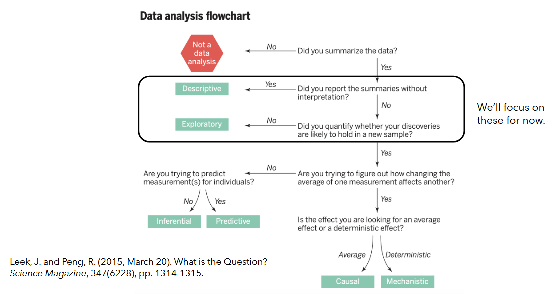
- our goal is to generate useful analyses
Exploratory Data Analysis...
- requires you to...
- investigate: get a first look of the data
- understand - gain an understanding of the data and its properties
- hypothesize - form new hypotheses and ask more questions for additional data collection and experiments
- involves...
- Summary Statistics - measure of central tendency, measure of dispersion, etc.
- Data Cleaning - fixing inconsistencies, removing invalid records, handling missing values.
- Data Visualization - scatterplot, dot plot, histogram, box plot
Some things to find out in the process of the EDA:
these are like guidelines or goals you might want to achieve in the process of the EDA
- different information that are available in the data
- range of values of each variable
- distributions of different variables
- presence of outliers, if any
- comparisons between different variables
- comparisons between groups of observations
- testing of personal assumption about the data
Regarding the format and the metadata
- What does each observation represent?
- What does each variable represent?
- Can i treat each row as individual records? Are there duplicates?
- Are there missing data to consider?
- What is the unit of measure for each variable?
- meta data is the data about the data → summary statistics, number of observations, how many variables, etc.
- duplication might be intentional
- unit of measure: metric? american?
Regarding the domain
- What do the terms/jargons in the dataset mean?
- In Financial Trading data - bid volume, bid-ask volume misbalance, signed transaction volume, spread volatility, bid-ask spread
- In Epidemiology data - basic reproduction number, generation time, incidence, serial interval, vaccine efficacy
- quantitative financial grading....?
- epidemiology: how do viruses spread...?
- familiarize yourself with the jargon if you're working with that kind of data
Regarding the Method of Collection
- Is the dataset a population or a sample in the context of the research qusetion?
- Are the possible biases in the dataset?
- Is the data collection consistent across all observations?
- Is it grouped?
- Is it simulated?
- ...Are there underlying groups? Is the data simulated from what is being drawn?
Regarding previous processing involved
- Are there previous processing performed on the data?
- Normalization - numerical values have been normalized to a set range?
- Discretization - numerical data has been grouped together into categories?
- Interpolation - are some values estimated from others?
- Truncation - some observations have been removed?
if you're working on large real world data, sometimes there are pre-processed datasets (cleaner) or raw datasets (if you have another cleaning method in mind)
Regarding the data itself
- Describe each variable in the dataset
- Summary statistics, frequency tables, histograms, etc.
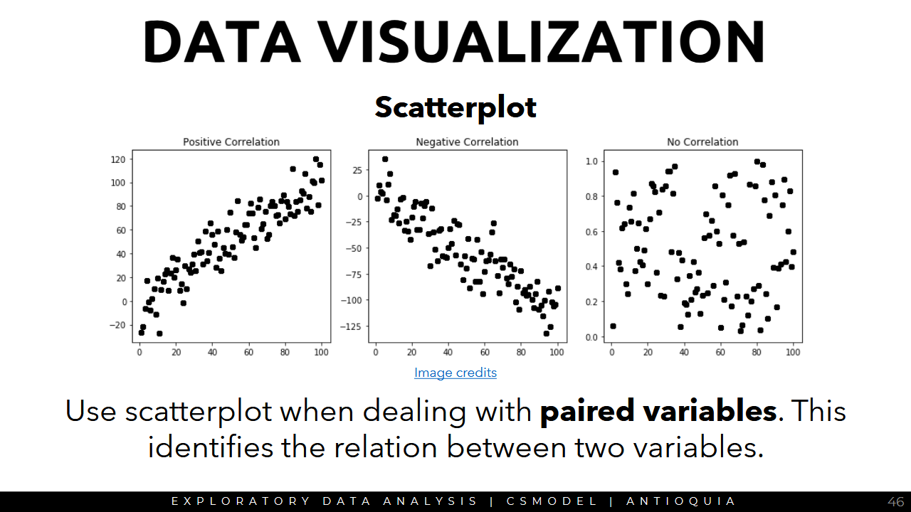
- Describe the relationship between pairs of vairables
- Scatterplots, correlation tables, etc.
Regarding each variable
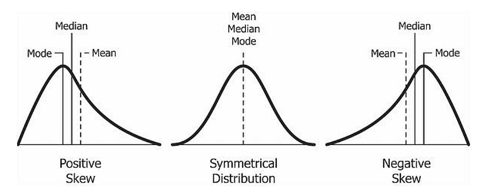
- What is the measure of central tendency? (mean, median, mode, trimmed mean, etc.)
- What is the measure of dispersion? (range, IQR, standard deviation)
- What does the distribution look like? (symmetric, positively skewed, negatively skewed, etc.)
Regarding relationships between variables
- Is there a relationship between two variables?
- Measures of correlation (Pearson, Spearman, etc.)
- Scatterplot, correlation tables, etc.
- Use the
corr()function in pandas for this (Pearson by default, check documentation)
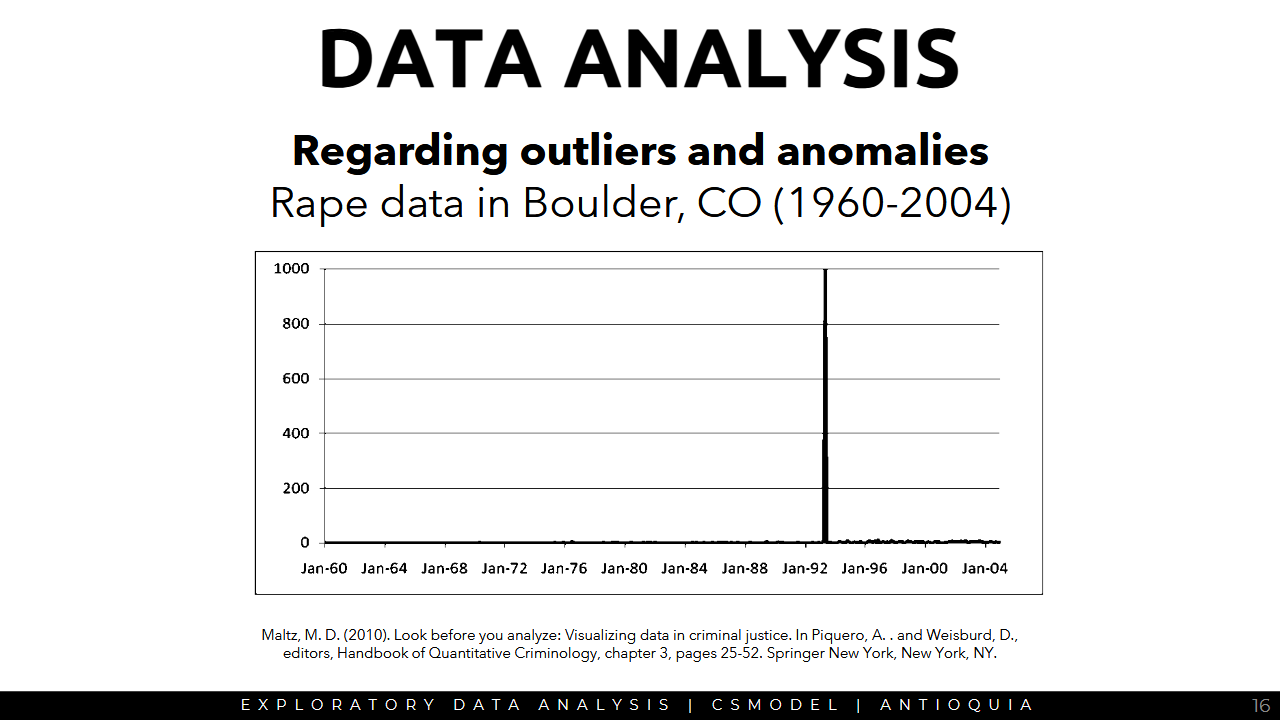
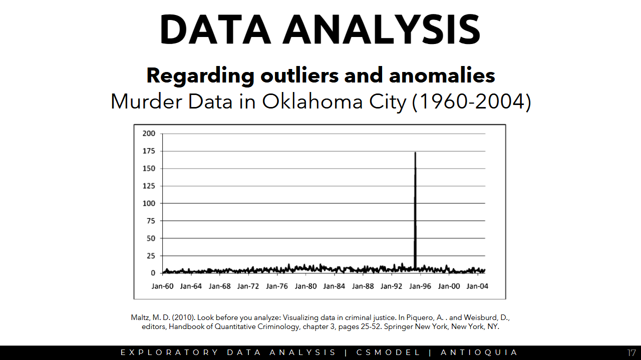
Regarding outliers and anomalies
- Are there outliers? Errors in encoding?
- Are there needed preprocessing steps to visualize and process the data properly?
Sample Data Visualization
Regarding additional Columns
- Are there additional columns to add to the dataset?
- Computed Index
- Poverty index
- H-index
- BMI
- Feature Pairs
- Male + old
- Cough + fever
- Generated Features
- Nearest grocery
- time duration
- date difference
Summary Statistics
Measure of Central Tendency
- Mean: add all the points, divide by the number of points (average)
- Trimmed Mean
- Median: middle value
- if tie, take the mean of the 2 middle values
- Mode: most occurring value
Example
54, 54, 54, 55, 56, 57, 57, 58, 58, 60, 60
- Mean = 56.6
- Median = 57
- Mode = 54
Mean
- Advantages: for both continuous and discrete numerical data
- Disadvantages: cannot be used for categorical data, easily influenced by outliers (super high/low value will drag the mean up/down)
Trimmed Mean
same as mean but removes the n% of the highest and lowest values in the dataset
- Advantages: for both continuous and discrete numerical data
- Disadvantages: cannot be calculated for categorical data
- addresses the problem of outliers but removing datapoints may have advantages/disadvantages
Median
the value separating the upper half and lower half of the sample/population
- Advantages: less affected by outliers and skewed data than mean, preferred when distribution is non-symmetrical
- Disadvantages: cannot be calculated for categorical data
- used in statistical inference and hypothesis tests
- Many ML stuff uses mean more than median, there's a deeper calculus analysis-related reason but sir doesn't have it lmao
Mode
most frequently occurring value in the sample/population
- Advantages: for both categorical and numerical data
- Disadvantages: may note reflect the center of the distribution very well. when the data is continuous, it may have no mode at all
Measures of Dispersion
- how far the data points are from each other
Range
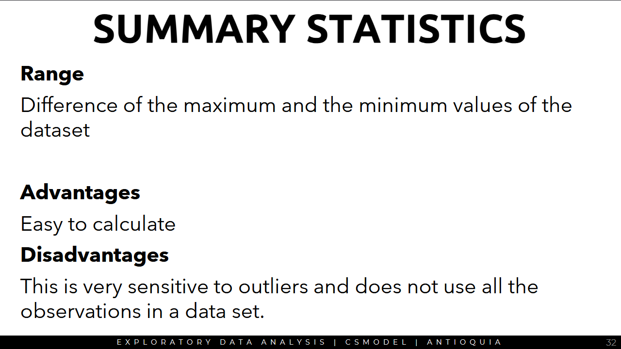
Interquartile Range
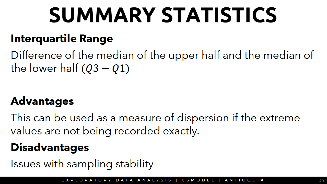
- lets say you have an equally distributed range of data from 0 to 100. assume the median Q2 to be 50. you want to look for Q1 (the median of the lowest value and the median Q2) = 25. Q3 is the median between overall median Q2 and upper bound Q3 = 75.
- interquartile range is Q3 minus Q1 (the 4th quartile is the maximum value =100)
- quartile just means 25% of the data/range of values
- if it's in the first quartile, it would be within the lower 25%, if it's in the second quartile its within 25-50% lower values.
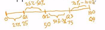
- the lower the quartile, the higher the rank
- adv: less susceptible to outliers
- sampling stability: the interquartile range might not be consistent among all the samples even though its from the same population
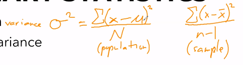
Standard Deviation
- sqrt of the variance
- Advantages: based on every item in the distribution
- Disadvantages: can be impacted by outliers and extreme values
variance: sigma squared
- the summation of the particula
- for each point, subtract it by the mean mu and square it
- n-1 if it's the sample variance, N if its the population variance
- mu is for population mean, x bar is for sample mean
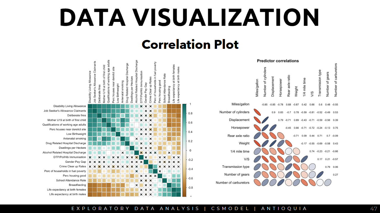
Correlation
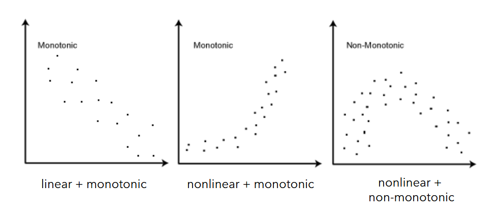
Pearson Correlation
assesses the linear relationship between two variables
Spearman Correlation
- Assesses the monotonic relationship between two variables (whether linear or not)
Data Visualization
matplotlibis a package for data visualization in Python that works well withpandas.- use it for visualizing data, which is an important step in EDA
Types of Plots
Scatterplot
Correlation Plot
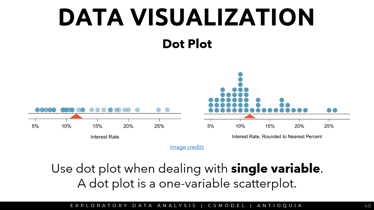
Dot Plot
Histogram
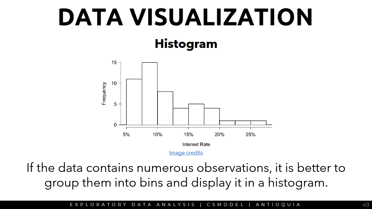
- Histograms provide a view of the data density and can be used to identify modes
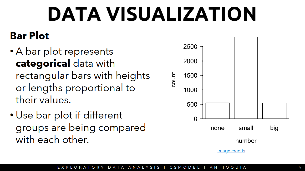
Bar Plot
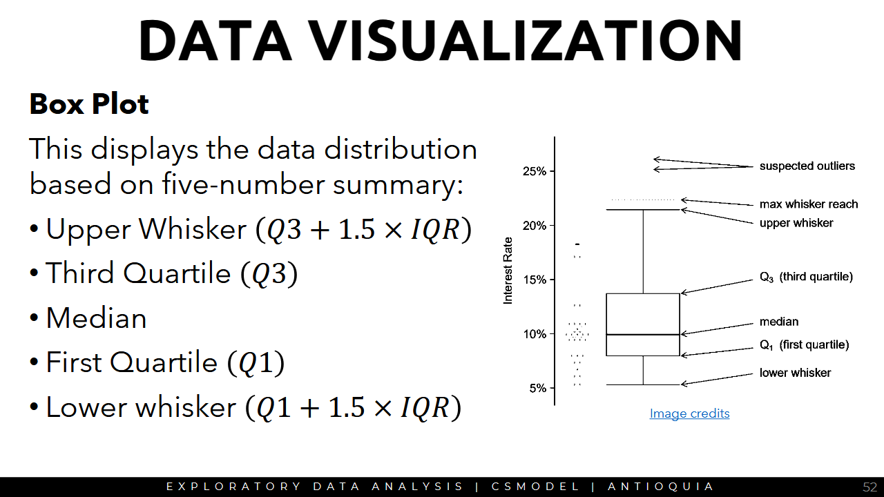
Box Plot
3a Foundations for Inference 🔴
Normal Distribution
Point Estimate
Confidence Intervals
Hypothesis Testing
Probability Distribution
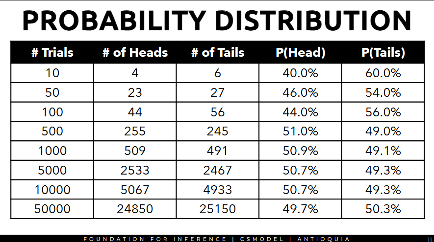
- the probability distribution represents the probabilities of different possible outcomes for an experiment
- to predict a variable accurately, understand the underlying behavior of the target variable first
- thus, knowing the probability distribution of the target variable is necessary
to get the probability distribution of the target variable, repeat the experiment numerous times, then record the number of times each outcome occurred.
- the probabilities of all outcomes should ∑ to 100%
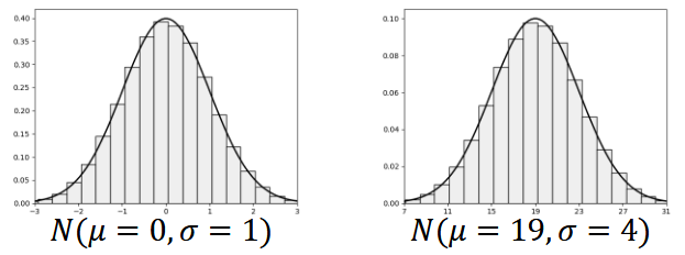
Normal Distribution
- a ubiquitous distribution that we see all throughout statistics
- bell-shaped curve, symmetric, and unimodal (there's only one high point)
Parameters of a Normal Distribution
- Mean (mu, μ) - center of the distribution
- standard deviation (sigma, σ) - spread of the distribution
- lower std dev → wider, fatter curve
- std deviation isn't the number of gaps necessarily or number of intervals. for visualization, you can use it as the size of the bin but it's not always the case
- it's a measure of how far apart your data is → the smaller, the close the variables are to each other
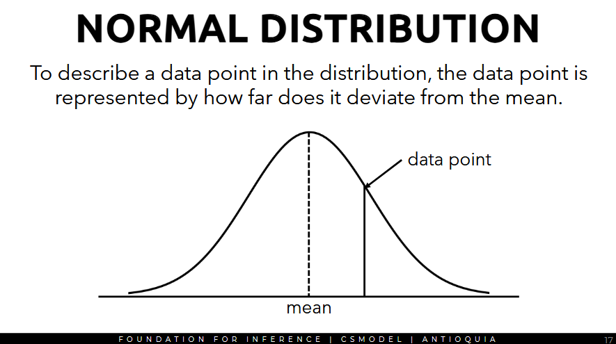
- to describe a data point in the distribution, the data point is represented by how far does it deviate from the mean
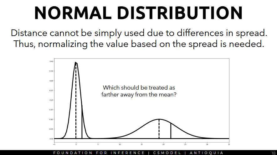
- distance cannot simply be used due to differences in spread, thus, normalizing the value based on the spread is needed.
- the dotted line is the mean, the solid one is the datapoint.
- the one on the right is farther away from the mean.
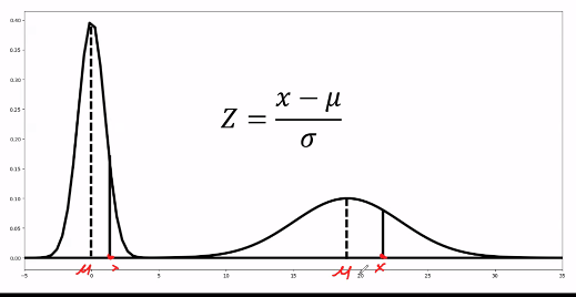
- we can answer this question using the z-score.
The z-score
- a standardized measure of how far a data point is from the mean
- a lower standard deviation would result in higher z-scores, while a larger standard deviation results in lower z-scores.
Percentile of a Data Point
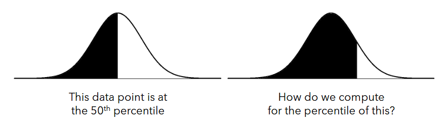
- the percentile of a data point corresponds to the fraction that lies below that datapoint.
- the 50th percentile is the same as the median
- 25th percentile is Q1, 75th is Q3
- percentiles should be within a range of 1 to 100
- percentiles may be used for determining rank
Computing for Percentile
- you can calculate the percentile in the previous picture via calculus, more specifically definite integrals: get the integral from negative ∞ to whatever x value
- computing for percentiles is essentially computing the area under a curve, which can be achieved with definite integrals, but in stats, we use tables.
- the z-score table has the z-score on the left.
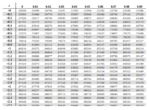
- if you have a z-score of 1.38, you want to compute the percentile. on the table this is approx 91.6th percentile
- if you have the 75th percentile, what's the z-score? would be approx 0.67
- the 25th percentile is just the negative of the 75th percentile, so you can just negate it because it's symmetrical
- the table assumes that the mean μ = 0 and standard deviation σ = 1, but you can customize it in python.
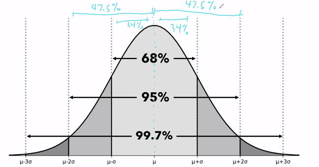
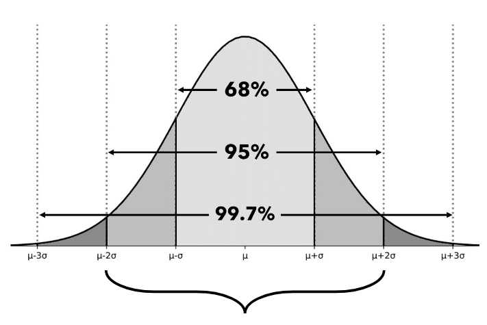
- visualization of the area under the curve wrt standard deviation and mean
- the top interval is 68% of the data, then 95%, then 99.7% and so on.
- the distribution is symmetric at the mean.
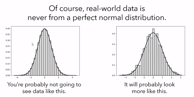
- most data seems to follow the normal distribution, but they're not perfect
- even though the data is not perfectly normal, normal distribution can be used to approximate it.
- the normal distribution is a mathematical model that approximates the data, rather than a direct property of the data.
Normal Distribution Formula
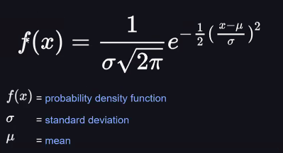
we use the normal distribution formula to approximate the data if the data is nearly normal.
- the data may look normal in a histogram plot, and the Normal Q-Q plot is mostly straight
- otherwise, using the normal distribution may lead to non-representative results
e: "Euler's number, denoted as "e," is a mathematical constant approximately equal to 2.71828. It is the base of natural logarithms and is widely used in mathematics, particularly in calculations involving growth and decay, such as compound interest."
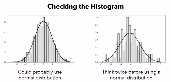
Checking the Histogram
- to check if the data is normally distributed, plot it into a histogram
Checking the Q-Q Plot (Quartile-quartile Plot)
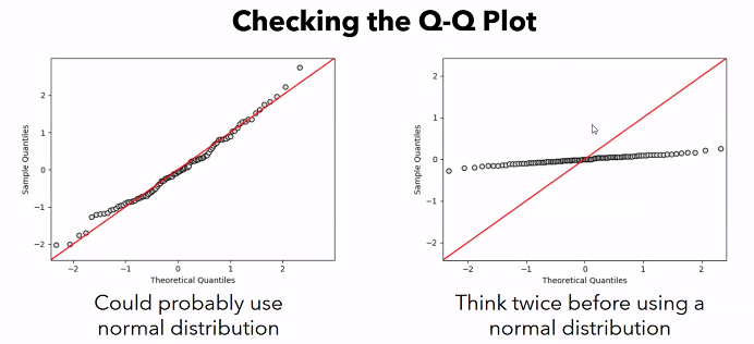
- assume it's a z-score.
- on the x-axis, compute the z-score for each observation assuming it was a normal distribution w mean=0 stddev=1 (normal), compute it with respect to the actual mean and stddev of the sample
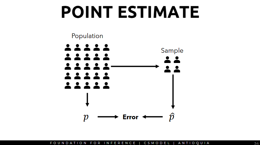
Point Estimate (p̂)
Example:
In the Dec2019 SWS survey, the PH president had an 82% satisfaction rating. This value is obtained from a sample.
- 82% is a point estimate (p̂) of the population parameter p
- The population parameter in this case is the actual satisfaction rating of the entire population, which we cannot directly compute because we don't have that data.
Types of Error
- Bias: Introduced in data collection process over or underestimation of true value
- Addressed through thoughtful data collection process
- Sampling Error: the variation of the estimate between different samples (our focus)

Suppose there is a very large population wherein all cannot be surveyed. We get a point estimate by surveying a small sample from the large population and get its approval rating (what we're trying to measure)
Repeat the sampling process multiple times and survey each sample to get its approval rating.
- the distribution of these point estimates is the sampling distribution, and its spread is the standard error.
Central Limit Theorem (CLT)
- the central limit theorem states that when observations are independent and the sample size is sufficiently large, the sampling distribution of the point estimate of certain statistics (e.g. proportion, mean) tends to be normally distribution
- if the population is normally distributed, then even low sample will make Central Limit Theorem hold.
- If not, the sample size of at least 30 is the general rule of thumb.
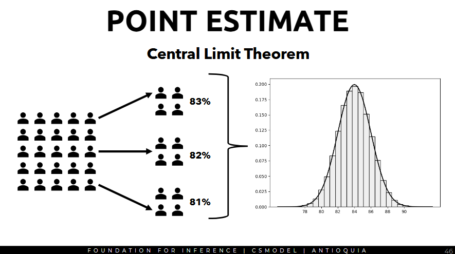
For proportion, the sampling distribution will be a normal distribution with:
- Means: p (population proportion)
- Standard error: sqrt(p(1-p)/n)
- Proportion is being used as an example, but same concepts will be expanded to other statistics in other examples.
Confidence Intervals (p49)
- it's difficult to hit the actual population proportion using a point estimate just from a single sample. thus, a single value might be insufficient. instead, a confidence interval is reported.
Example: In the December 2019 SWS survey, the satisfaction rating of Pres. Duterte is 82 ± 3% with a 95% confidence level
To construct a confidence interval with 95% confidence, we do
- where SE is the standard error
- since 95% of the data lies within 1.96 standard deviations from the mean.
Intuition
- If sampling is repeated many times, expect that the confidence interval would contain the true population population proportion 95% of the time
- if the confidence level is 95%, and there are 20 independent samples, then the confidence intervals from 19 out of 20 independent samples contain the actual proportion
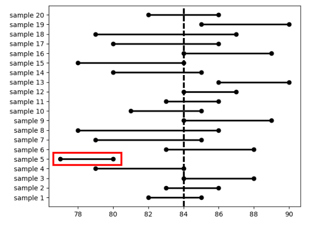
- so the red part is the actual proportion (double check)
Increasing the confidence level to 99%:
Hypothesis Testing
confirms if the hypotheses are true in a statistically significant way based on the sample data
Process
- State null and alternative hypotheses
- Decide on test statistic and compute the p-value
- Decide based on the p-value
Example
Pew Research asked a random sample of 1k American adults whether they supported the increased usage of coal to produce energy. The sample of 1000 American adults show that 37% of American adults support increased usage of coal.
Set up hypotheses to test if majority of American adults support or oppose the increased usage of coal.
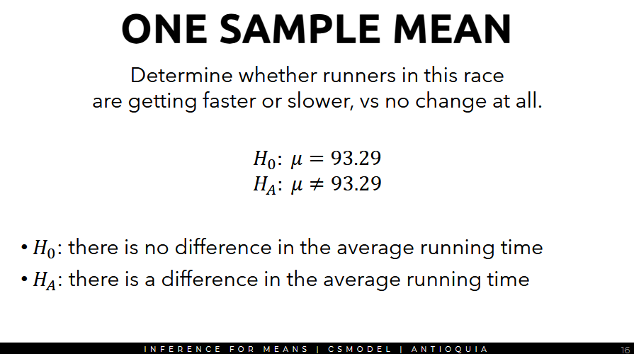
Null and Alternative Hypotheses
- The null hypothesis (H_0) often represents a skeptical perspective or claim to be tested
- The alternative hypothesis (H_A) represents an alternative claim under consideration and is often represented by a range of possible parameter values.
- Data scientists should play the role of a skeptic: to prove the alternative hypothesis, a strong evidence is needed.
- Guilty until proven otherwise
Example Cont
Set up hypotheses to test if the majority of American adults support or oppose the increased usage of coal.
Null: There is no majority, i.e. p = 0.5
Alternative: There is a majority support or opposition (though we do not know which one) to expanding the use of coal
the sampling distribution should look like this if the null hypothesis is true:
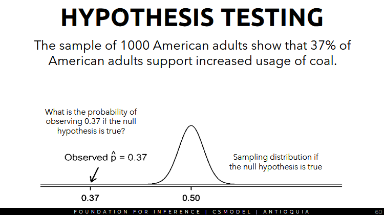
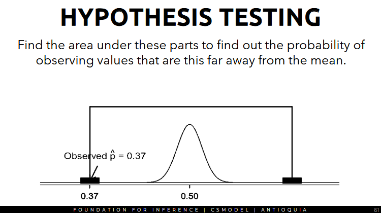
- we want to find the area under these parts to find out the probability of observing values that are this far away from the mean
Z-score and z-test
to perform hypothesis testing for proportion, compute the Z-score and use the z-test.
- the p-value is the probability of obtaining results at least as extreme as the observed results of a statistical test, assuming the null hypothesis is correct
- using the computed z=score, the p-value is 4.4 * 10^-16 ≈ 0.00000000000000044
The significance level is the p-value in which you decide to reject the null hypothesis. (threshold whether to reject or not)
- common significance levels α = 0.01, 0.05, 0.1
- otherwise accept the null hypothesis
Since the p-value (4.4 * 10^-16) is less than the significance level 0.05, so we reject the null hypothesis. thus, there is a majority support or opposition to expanding the use of coal.
Summary of what we did
- get the p-value based on the z-value (-8.125). the p-value is 4.4 * 10^-16
- using significance level 0.05, the p-value 4.4 * 10^-16 is statistically significant
- since the p-value (4.4 * 10^-16) is less than the significance level 0.05, reject the null hypothesis
Types of Decision Errors
Statistical test can potentially make decision errors.
- Type 1: null hypothesis is true, but is interpreted as false
- Type 2: null hypothesis is false, but is interpreted as true
Summary
- Normal distribution is a common type of distribution in statistics and the highlight of the Central Limit Theorem
- CLT (Central Limit Theorem) notes that when certain conditions are met, the sampling distribution of the point estimates will be normally distributed and can estimate the true parameters of interest.
3b Inference for Means 🔴
T Distribution
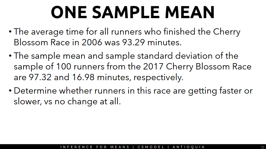
One Sample Mean
Paired Observations
Unpaired Observations Multiple Means
Parametric Test
- coming from the name, parametric tests assume that the parameters and the distribution of the population is known
- the comparison is done between the mean or the measure of central tendency
- these tests require that you know the distribution of your data and that the sample population fits the assumed distribution of the test
- earlier we assumed the data was normally distributed
Prerequisite: Central Limit Theorem
- When collecting a sufficiently large sample of 𝑛 independent observations from a population with mean μ and standard deviation σ, the sampling distribution of sample mean x^bar will be nearly normally distributed, with mean μ and standard error σ / sqrt(n)
- If population is normally distributed, then even low samples will make CLT hold. else, a sample size of at least 30 is a general rule.
If the sample size is small, this estimate for the standard deviation:
- becomes problematic so we use t-distribution instead of a normal distribution
TLDR; using standard error is problematic if the sample size is small so t-distribution is the alternative
GEMINI: Standard Deviation tells you how "diverse" the individuals are in your group (sample). Standard Error tells you how "diverse" the average of your group would be if you repeatedly picked different groups from the same population.
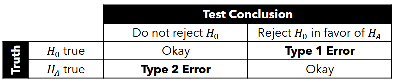
T-distribution
- the graph of a t-distribution has thicker tails
- more effective in approximating the sampling distribution of sample mean xbar
- like the z-score, it is a standardized way to determine how far the observation is from the mean
- where x is the observation
- xbar is the sample mean
- divided by standard error, where n is the number of observations
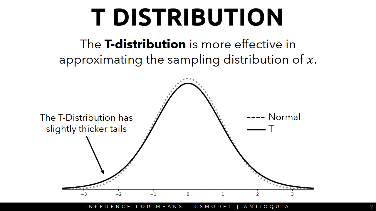
Degrees of Freedom
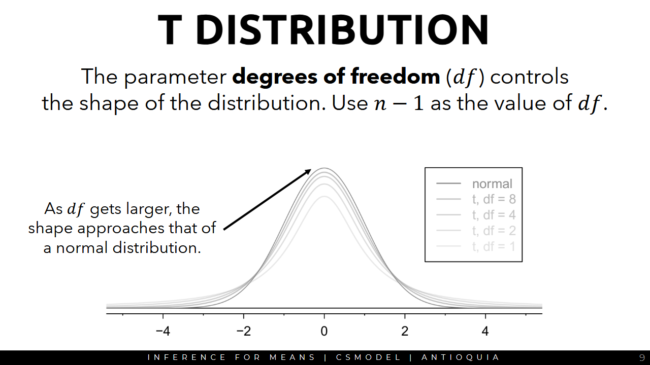
- degrees of freedom df is the number of independent variables
- darkest line is the actual normal distribution
- other lines are varying degrees of freedom
Confidence Intervals
Example
Given n = 19 instances, sample mean x̄ = 4.4, sample standard deviation σ = 2.3
df = n - 1 = 19 - 1 = 18
- To construct a confidence interval with 95% confidence, get the z-score of the point where 95% of the observation will fall (using the t-table)
- Multiply the z-score with the standard error s/sqrt(n)
- Confidence interval is the result ± x̄ with a 95% confidence level
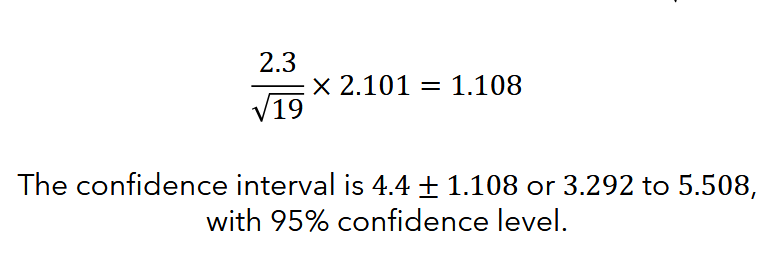
- When sampling is repeated many times, confidence interval will contain the true population mean 95% of the time.
One Sample Mean and One Sample T-test
- it's one sample mean bc we're only taking one sample and only focusing on that sample
- we want to determine if the mean of that sample can be within the actual mean
To confirm if the hypotheses are true in a statistically significant way, we perform hypothesis testing.
Since observations are independent and n ≥ 30, use the t-distribution to estimate the sampling distribution of the mean where df = 99
To perform hypothesis testing for mean, compute the T-score and use the T-test
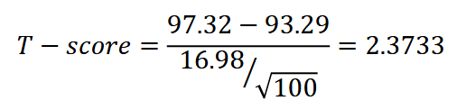
Then, using the t-table, get the p-value based on the T-score (2.3733) and df=99. the p-value is 0.0195.
Using significance level α = 0.05, the p-value is less than the significance level 0.05, reject the null hypothesis
thus, the data provides strong evidence that the average run time for the Cherry Blossom Run in 2017 is different than the 2006 average at a significance level of 5%
Paired Observations
- used for when each observation is associated with two variables
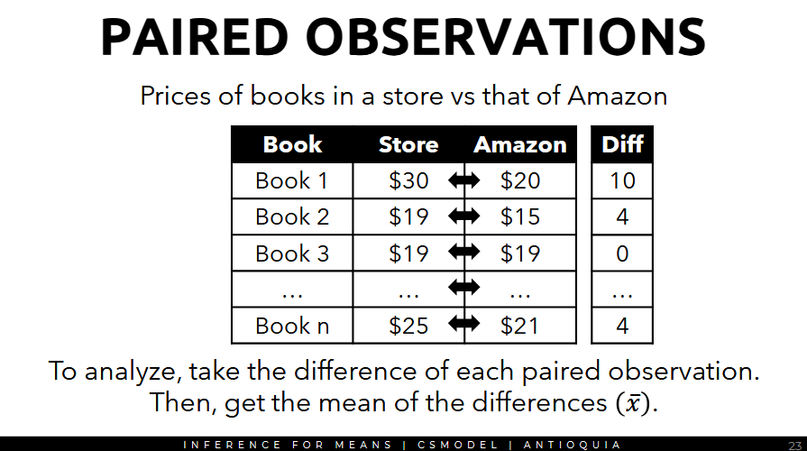
Perform analysis on the difference between paired observations.
- n = 68
- μ_d = 3.58 (mean of the differences)
- s = 13.42 (standard deviation)
Since the data is independent and n = 68, apply CLT even though the distribution is not normal.
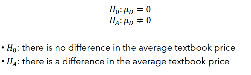
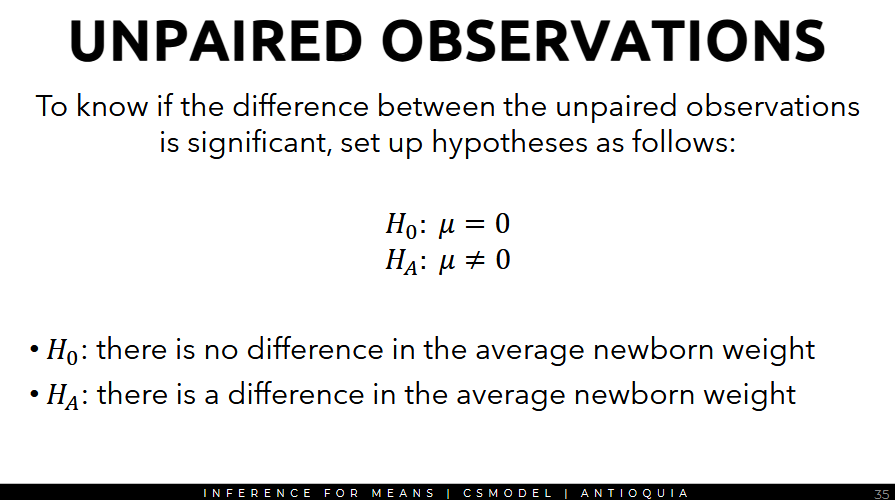
To know if the difference between the paired observations is significant, set up the hypotheses as two-tailed tests.
We're using the Standard Error for the mean of a single sample.
To perform the hypotheses testing, compute the T-score of the observed mean of the differences and use the T-test
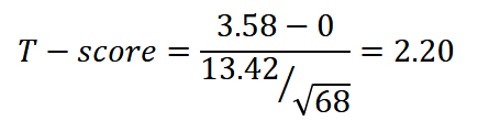
Then, using the t-table, get the p-value based on the T-score (2.20) and df (67). The p-value is 0.0312.
Using significance level α = 0.05, the p-value is statistically significant.
since the p-value is less than the significance level, reject the null hypothesis.
thus, the data provides strong evidence that the prices in the store are different than that of Amazon at a significance level of 5%
Unpaired Observations
- use when you're comparing two groups that aren't paired, sample size may not be necessarily the same
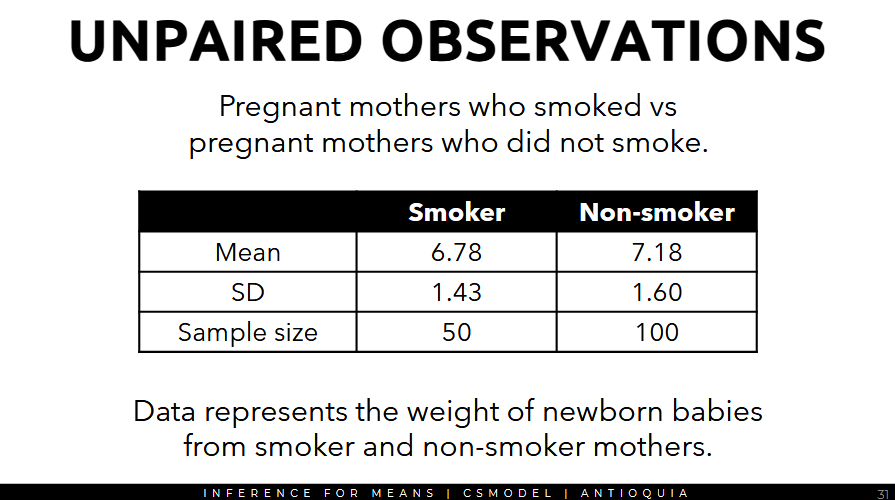
calculate the point estimate for the mean as 7.18-6.78 = 0.40
Then setup the hypotheses
Given 2 separate groups, consider the estimates for the mean difference sampling distribution
Here, we're using the Standard Error of the Difference Between Two Independent Means
set df to the lower sample size - 1
- t-distribution df = 49
To perform hypothesis testing, compute the T-score of the point estimate and use the T-test
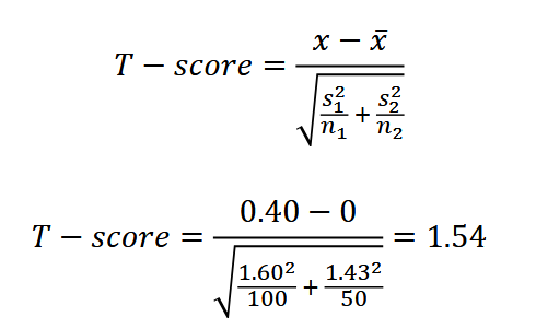
Then, using the t-table, get the p-value based on the T-score (1/54) and df (49). The p-value is 0.135.
Using significance level α = 0.05, the p-value (0.135) is statistically unsignificant. Since the p-value is greater than the significance level α, accept the null hypothesis.
Thus, the data provides strong evidence that there is no difference between the weights of newborns from smokers and non-smokers at a significance level of 5%
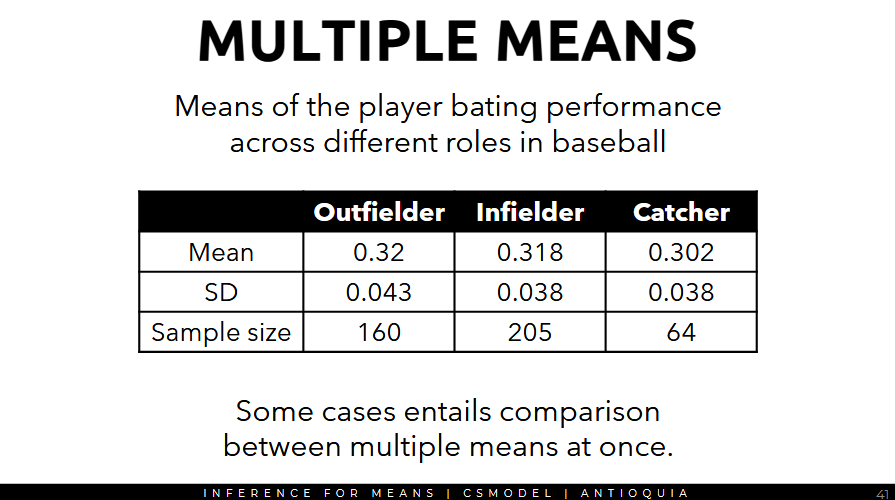
Multiple Means and ANOVA F-statistic
- some cases entails comparison between 2+ means
ANOVA Core Concept: if the means are the same, then their variability should be low.
Setup the hypotheses
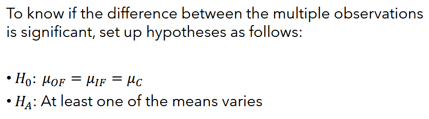
ANOVA Computes for the F-statistic
- where MSG is Mean Square between Groups (measure of variability between groups)
- where MSE is Mean Square Error (variability within each group)
F-Distribution (df1 and df2)
df1 = k - 1where k is the number of groupsdf2 = n - kwhere n is the total sample size across all groups
To perform hypothesis testing, use the F-statistic
Get the p-value based on the F-statistic (5.077). The p-value is 0.006
Using significance level α = 0.05, the p-value 0.006 is statistically significant.
Since the p-value is less than the significance level, reject the null hypothesis.
Thus, the data provide strong evidence that at least one of the groups deviates from the others under a significance level of 5%
To find out which group, we can compare all pairwise means using the method previously shown (outfielder VS infielder, outfielder VS catcher, infielder VS catcher), but we need to apply a Bonferroni correction to account for increased chances of a Type 1 error.
- where a is the original significance level
- where K is the number of comparisons made
(more comparisons mean higher chances of making mistakes, if α = 0.05, then there is a chance of making a Type 1 error 5% of the time)
Use the intuitions behind CLT to establish statistical significance when comparing means.
Use the t-distribution to estimate the sampling distribution of the means taken from some population.
Determine the probability that a value as extreme as the observation can be observed from the sampling distribution of our null hypothesis to know its significance.
Use ANOVA to compare the means of multiple groups at once.
3c Inference for Categorical Data 🔴
Test of Goodness of Fit
Test of Independence
Recap of Statistical Testing
Example
Test the hypothesis that there is a difference in the average sleeping time of boys and girls. Take a sample of the population. Compute the desired statistic from the sample. In this case, the difference between the means/average.
Suppose that the difference between the average sleeping time of boys and girls is 1.6 hours. Find out if this observation is statistically significant.
Assume the null hypothesis is true: there is no difference in the mean sleeping time (mean difference = 0)
based on the Central Limit Theorem...
taking multiple samples repeatedly results to a sampling distribution that can be approximated with t-distribution
- one of the samples has a difference of 1.6 hours.
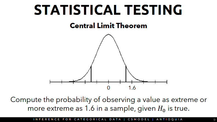
Compute the probability of observing a value as extreme of more extreme as 1.6 in a sample, given that the null hypothesis is true.
If the probability (p-value) is small, then there is some evidence to believe that the null hypothesis is likely not true.
Otherwise, since the probability of observing that value in a sample is high, then we cannot say that the null hypothesis is likely to be false.
Steps in Statistical Testing:
- Compute some statistic from the sample.
- Determine the sampling distribution of that statistic if the null hypothesis is true.
- Check the probability that the sample statistic could be observed from the distribution.
- Reject the null hypothesis if the probability is low enough.
Test of Goodness of Fit (Chi-Square Test)
- Goodness of fit: used to test whether the sample is representative of the general population
- observations in the dataset should be classified into different groups.
- stratified random sampling → testing goodness of fit would be a good choice if your sample is appropriately stratified
Example
| Race | White | Black | Hispanic | Other | Total |
|---|---|---|---|---|---|
| Juries | 206 | 26 | 25 | 19 | 275 |
| Voters | 72% = 0.72 | 7% = 0.07 | 12% = 0.12 | 9% = 0.09 | 100% |
| Expected | 275 * 0.72 = 198 | 265 * 0.07 = 19.25 | 265 * 0.12 = 33 | 265 * 0.09 = 24.75 |
For context:
- juries randomly select from citizens of a country so they could participate
- if you're part of a jury you have to attend the trials and they should unanimously decide if the defendant is guilty or not
Q: is the number of juries per race representative of the actual population?
- the data of the race distribution of the registered voters can be used as reference for the ideal distribution.
- the ideal number of people in each race in the jury can be computed using the percentage of voters as reference.
- we use that to calculate the expected numbers.
Given the expected counts, check if the observed counts are statistically different from the expected distribution or is the difference likely a result of chance.
Define the null and alternative hypotheses:
- Null: the jurors are a random sample, i.e., there is no racial bias in who serves in a jury.
- Alternative: The jurors are not randomly sampled, i.e. there is racial bias in juror selection.
Here, we use the Chi-Square test, if the following are met:
- each observation in the table should be independent of all other observations
- each expected count should be at least 5
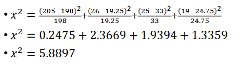
- We take the difference of the observed counts, subtract by expected counts, squared difference, divide by expected count for the particular group → you do this formula across all four ethnicity groups
- top: how far is the observed count from the expected count?
- expected_i: normalize it according to the group size.
- when you do chi-squared alone: if the chi2 value is close to 0, then it seems to be a good fit
- if it's a larger value, then it's evidence that the observed value doesn't really fit the expected value
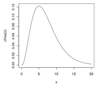
Chi-Square Distribution
The Chi-Square distribution is the expected distribution of the Chi-Square statistic when you take repeated samples from a population
- assuming there's no racial difference, then the chi2 statistic distribution should look something like this:
Parameters of Chi-Square Distribution
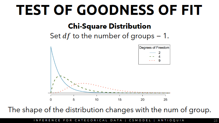
Degrees of freedom is another parameter in the Chi2 Distribution
- StatisticsByJim: Degrees of freedom are the number of independent values that a statistical analysis can estimate. df for chi-square = (rows -1) (cols - 1)
- rows: 2 (observed and expected)
- cols: 4
- df = (2-1)(4-1) = (1)(3) = 3
- the blue solid line is the chi2 distribution if there are 2 degrees of freedom for 3 groups
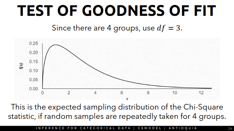
- we have 4 groups so we use df = 3, and that's what the chi2 distribution should look like.
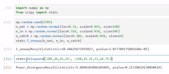
Q: What is the probability of observing a value as extreme as x^2 = 5.8897 or more, given our expected distribution?
- use
stats.chiquare, first param is the observed value, second one is the expected values
Steps for performing a hypothesis test (specifically a chi-square goodness-of-fit or chi-square test of independence):
- Get the p-value based on the chi-square value of 5.8897 and df = 3. The p-value would be 0.1171
- Use a significance level α = 0.05, the p-value is not statistically significant because the p-value is higher (SimplyPsychology: a p-value less less than or equal to your significance level IS statistically significant)
- Since the p-value 0.1171 is greater than the significance level, fail to reject the null hypothesis.
- Thus, the data provides strong evidence that the juror are randomly sampled and there are no bias in juror selection at a significance level of 5%.
Another Example:
| Age Group | 18 to 39 | 40 to 59 | 60+ | Total |
|---|---|---|---|---|
| Respondent | 702 | 398 | 100 | 1200 |
Q: Is the number of respondents per age group representative of the actual set of registered voters?
- the data of the age group distribution of the registered voters can be used as reference for the ideal distribution.
- the ideal number of people of each age group can be computed using the percentage of voters as reference
| Age Group | 18 to 39 | 40 to 59 | 60+ | Total |
|---|---|---|---|---|
| Respondent | 702 | 398 | 100 | 1200 |
| Voters | 56% | 32% | 12% | 100% |
| Expected 18-39: 1200 * 0.56 = 672 | ||||
| Expected 40-59: 1200 * 0.32 = 384 | ||||
| Expected 60+: 1200 * 0.12 = 144 |
| Age Group | 18 to 39 | 40 to 59 | 60+ | Total |
|---|---|---|---|---|
| Respondent | 702 | 398 | 100 | 1200 |
| Expected | 672 | 384 | 144 | 1200 |
| Given the expected counts, check if the observed counts are statistically different from the expected distribution or is the difference likely just a result of chance. |
Determine the null and alternative hypothesis:
- Null: The respondents are a random sample and are representative of the current set of registered voters.
- Alternative: The respondents are not randomly sampled and are not representative of the current set of registered voters.
Compute x^2 for the Chi-Squared Test:
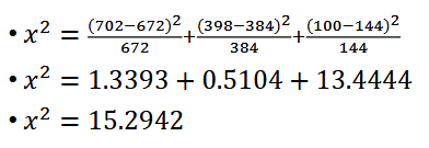
- Get the p-value based on the chi-square value (15.2942) and df = 2. The p-value is 0.0012.
- Using significance level 0.05, the p-value 0.0012 is statistically significant.
- Since the p-value is less than the significance level, reject the null hypothesis.
- Thus, the data provides strong evidence that the respondents are not randomly sampled and are not representative of the current set of registered voters at a significance level of 5%
Test of Independence
Example Context: Pulse Asia Commissioned Survey by Senator Gatchalian
Q: The ROTC or Reserved Officers' Training Corps is a program which aims to teach the youth about discipline and love of country through military training. How much do you agree or disagree with the proposal to implement ROTC to all students in SHS?
- There are arguments that the phrasing of the question might be leading the survey participants, thus the result might not be reliable.
Revised Q based on RA 9163: ROTC is a program designed to provide military training to tertiary level students in order to motivate, train, organize, and mobilize them for national defense preparedness.
Q: How much do you agree or disagree with the proposal to implement ROTC to all students in SHS?
Some examples compare categorial responses between multiple groups. Group A got the original question, Group B got the negative version, Group C got the legal definition.
- We're testing if the phrasing of the question affects the response.
| Group | Group A | Group B | Group C |
|---|---|---|---|
| Agree | 23 | 2 | 36 |
| Disagree | 50 | 71 | 37 |
Test for independence checks whether two categorial variables are independent of each other. (which would be the null hypothesis)
- If they're truly independent, then the distribution of one variable should be the same across all categories of the other variable.
- Base the expected proportion according to the total
| Group | Group A | Group B | Group C | Total |
|---|---|---|---|---|
| Agree | 23 | 2 | 36 | 61 |
| Disagree | 50 | 71 | 37 | 158 |
| Total | 73 | 73 | 73 | 219 |
Get the proportion:
Agree = 61/219 = 0.2785
Disagree = 158/219 = 0.7215
Get the expected frequencies by multiplying to the total:
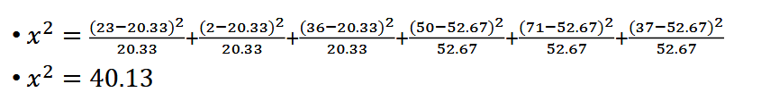
Agree = 0.2785 * 73 total = 20.33
Disagree = 0.7215 * 73 = 52.67
- Create the Null and Alternative Hypotheses
Null H_0: Responses are independent of the question, i.e. the phrasing did not affect the response
Alternative H_A: Responses are dependent on the question, i.e. the phrasing affects the response.
Chi-Square Test
- Conduct a Chi-Square Test to get the chi2 statistic for addressing the null hypothesis
Chi-Square Distribution
- Calculate for the degrees of freedom for the Chi-Square Distribution.
- Goodness of Fit doesn't really care about rows and columns. In test of independence, we use the unique responses.
- Total columns and row headings aren't considered
df = (rows - 1) * (cols - 1) = (2-1) (3-1) = (1)(2) = 2
- Based on the Chi-Square Distribution, what is the probability of observing the x^2 value (Chi-squared statistic) = 40.13? (i.e. we want to find the area under the curve)
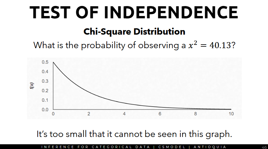
It's too small to be seen in the graph.
Test of independence steps:
- Get the p-value based on the chi-square value (40.13) and df = 2.
- The p-value is 0.000000002
- Using significance level α = 0.05, the p-value is statistically significant so we reject the null hypothesis. (in p-value, if value < 0.05, reject the null hypothesis)
- Thus, the data provides strong evidence that the answer of the respondents depends on the phrasing of the question.
In code (scipy.stats)
- chisquare is for goodness of fit
- chi2_contingency(array) is for test of independence
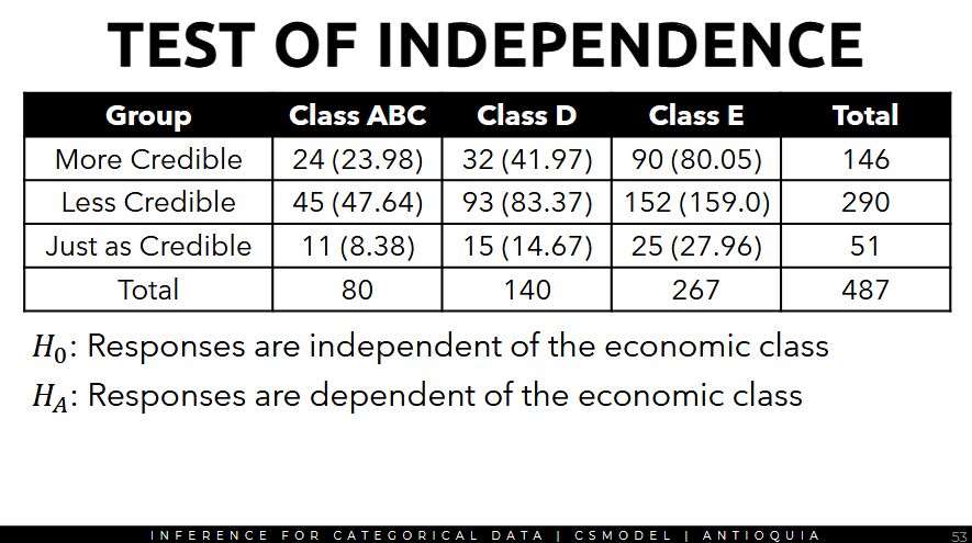
Example: Election results and Economic Class
| Group | Class ABC | Class D | Class E |
|---|---|---|---|
| More Credible | 24 | 32 | 90 |
| Less Credible | 45 | 93 | 152 |
| Just as Credible | 11 | 15 | 25 |
Q: is the answer of the respondent dependent on the economic class?
- Get the total
| Group | Class ABC | Class D | Class E | Total |
|---|---|---|---|---|
| More Credible | 24 | 32 | 90 | 146 |
| Less Credible | 45 | 93 | 152 | 290 |
| Just as Credible | 11 | 15 | 25 | 51 |
| Total | 80 | 140 | 267 | 487 |
- Calculate for the proportion and the expected values.
Proportion:
- More Credible = 147/486 = 0.2998
- Less Credible = 290/487
- Just as Credible: 51/487 = 0.1047
(Expected value is proportion * total)
Expected Values for More Credible
- Class ABC: 0.2998 × 80 = 23.98
- Class D: 0.2998 × 140 = 41.97
- Class E: 0.2998 × 267 = 80.05
Expected Values for Less Credible:
- Class ABC: 0.5955 × 80 = 47.64
- Class D: 0.5955 × 140 = 83.37
- Class E: 0.5955 × 267 = 159.00
Expected Values for Just as Credible:
- Class ABC: 0.1047 × 80 = 8.38
- Class D: 0.1047 × 140 = 14.67
- Class E: 0.1047 × 267 = 27.96
- Put them all together and create the Null and Alternative Hypotheses
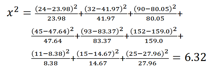
- Compute the Chi-square statistic to test the null hypothesis.
Steps
- Get the p-value based on the chi-square value (6.32) and df = 4
- the p-value = 0.1765
- With a significance level of 0.05, the p-value is statistically significant. (in p-value, if value < 0.05, fail to reject the null hypothesis)
- Thus, the data provides evidence that the responses are independent of the economic class.
Summary
- use the intuitions of hypothesis testing and (focusing on means of different groups) extend it to binned data (numerical data spread across different groups)
- compute the chi-square statistic, calculate the probability (p-value) that this statistic can be observed in the sampling distribution approximated by the appropriate chi-square distribution with param degrees of freedom
3d Bayesian Inference 🟠
Conditional Probability
Bayes Theorem
Two kinds of statistics
- Frequentist Statistics - focuses on the frequency or the proportion of the data
- most used technique in statistics
- the frequentist approach tests whether an event or hypothesis occurs or not
- probability is calculated based on many repetitions of the experiment and counting how many times the event occurs
- the result of the experiment is dependent to the number of times the experiment is repeated
- different p-values might be obtained using the same data but different stopping intention and sample size
- Bayesian Statistics - focuses on beliefs and updating those beliefs based on new data
Conditional Probability
- conditional probability is defined as the probability of an event A given that event B has already happened.
Example Scenario
Suppose out of all the 4 championship races between Niki and James, Niki won 3 times while James managed only 1. What is the probability that James will win?
Assume event B is that James won.
Total events = 4
P(B) = 1/4

Suppose out of all the 4 championship races between Niki and James, Niki won 3 times while James managed only 1. Out of the 1 time James won, it was raining. Out of the 3
times Niki won, it was raining only 1 time. If it was raining in the next race, what is the probability that James will win?
Assume event A is that it was raining, event B is that James won.
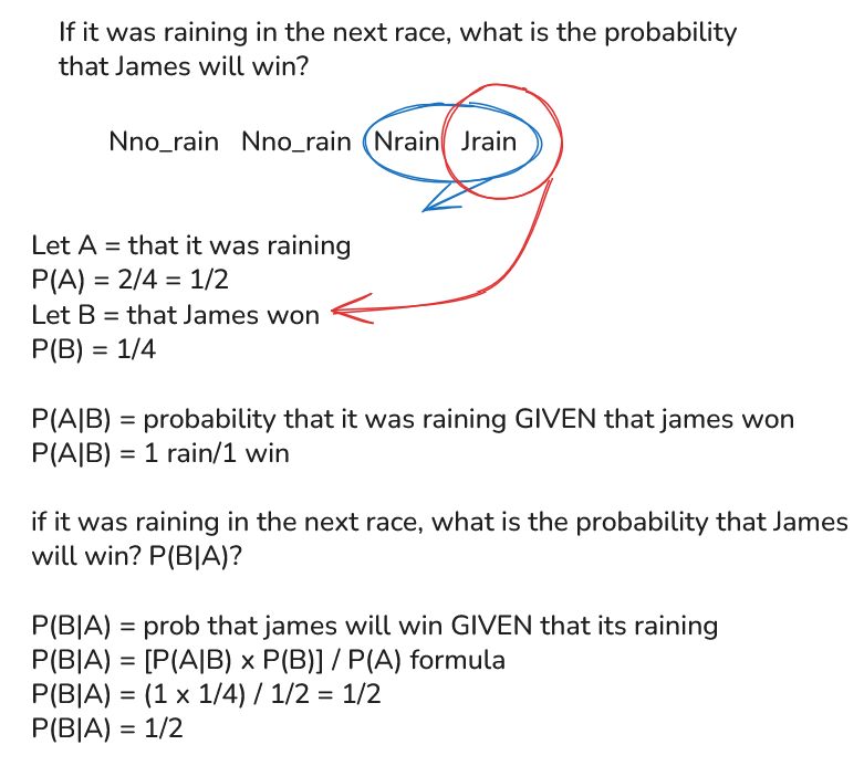
(Answer is correct)
The evidence of rain strengthened our belief that James will win the next race (doubled it.)
Bayes Theorem
- where A and B are events
- P(B) ≠ 0
- P(A) and P(B) are the probabilities of observing A and B respectively, they are also known as the marginal probabilities
Bayesian Inference
Dr. Trefor Bazett: Bayes' Theorem - The Simplest Case
Terms needed in Bayesian Inference (or inference in general)
Models: mathematical formulations of the observed events
- like a standard formula, step-by-step algorithms
Parameters: inputs that influence the model - like in normal distribution, the params are mean and standard deviation (or variance)
- in t-distribution, the parameter is degrees of freedom
Example Scenario:
Consider the task of flipping a coin, where heads is considered as the successful case and tails is considered as the unsuccessful case.
In this case...
let θ: a parameter to the model representing the fairness of the coin
let D: the outcome of the events.
ex. D could be either heads or tails, and θ is the probability of getting heads or tails in our coin
Given an outcome D, what is the probability that the coin is fair, i.e. θ = 0.5? (50% chance of getting heads)
- where P(θ): prior strength of the belief. this is the strength in the belief of θ without considering the evidence D.
- where P(D|θ): the likelihood of observing the result, given the distribution for θ. this is the probability of seeing the data D as generated by a model with parameter θ.
- where P(D): the evidence. This is the probability of the data as determined by summing across all possible values of θ, weighted by the strength of the belief to values of θ.
- where P(θ|D): the posterior belief of the parameter after observing the evidence. this is the strength of the belief of θ once the evidence has been considered. → what we're actually computing
Prior belief (before) --evidence→ Posterior belief (after)
- a mathematical model is needed to represent the prior belief and the posterior belief distributions
- both should have the same mathematical
Q: Is belief = confidence?
A: belief is whatever the conclusion is, confidence is how likely that belief would be true
The Bernoulli Function or Bernoulli Distribution Function
Bernoulli probability distribution function is one of the models
- use if you want to represent your data as a 0 or 1
- where y = 1 when the case is successful (heads)
- and y = 0 when the case is unsuccessful (tails)
Example
If you're working with financial data, and there's a guy who applies for a loan application. You want to predict if the guy will pay his payments on time or will he fail to pay.
- y=1 when he is trustworthy
- y=0 when he is not (i.e. fails to pay the loan)
Example
If you're in healthcare, y=1 when the person is positive for a diagnosis, y=0 when negative.
Bernoulli function computes the actual probability within 0 to 1, used when we have a assumed probability in mind.
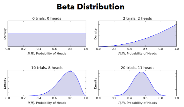
Beta Distribution
- Beta distribution can be used to represent prior distribution
- The Beta distribution can be used to model beliefs on a binomial distribution
- binomial distribution example: let's say you flip a coin 10 times. what's the probability of getting 7/10 heads? ← that's what the binomial distribution is trying to predict.
- Wikipedia: the binomial distribution is used to model the number of successes in a sample size n, drawn with replacement from a population of size N.
- Investopedia: the binomial distribution shows the probability that a value will take one of two independent values under a given set of parameters or assumptions. It assumes there is only one outcome for each trial, each trial having the same probability of success, and each trial is mutually exclusive or independent of the others.
- where α = number of desired/successful outcomes
- where β = number of undesired/failed outcomes
- and x = assumed probability, our guess for the probability (ranging from 0 to 1)
- B(α, β) = the Beta function, different from the Beta distribution
- Wikipedia: The Beta function is a normalization constant to ensure that the total probability is 1. It has a completely different formula, which isn't required in this course
Beta distribution can be helpful when you don't know what the probability is, but you have the set of observations. So it's useful in estimating what the likely probability is.
- we're trying to compute the likelihood of each head(?) happening
- density is like the score of the likelihood of our observations
- density (can reach higher values) ≠ probability (0 to 1)
- for 0 trials, 0 heads: if we have 0 trials, we can't estimate what the probability is regarding if the coin is fair or not → so every probability is equally likely.
- for 2 trials, 2 heads: we flip our coin two times and in both scenarios we get 2 heads.
- α = 2 success, β = 0 fails
- probability of heads = 1 is very likely, maybe around a likelihood of 70-80% density score (likelihood score)
- for 10 trials, 8 heads: we flip our coin 10 times and get 8 heads
- α = 8, β = 2
- the distribution shows us it's very likely that we will get heads at 60-80%, but no less than 60%
- for 20 trials, 11 heads: α = 11, β = 9
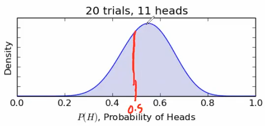
- the red mark is at the 50%, the highest density is at around 0.55
- we don't have to write this by hand in this course, scipy might have plots for this
More examples
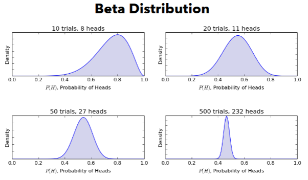
- the more you increase your α and β, the higher the likelihood score will be
We can also calculate the mean and standard deviation of a Beta distribution:
- Example in the quiz: you flip a coin 20 times and you get 11 heads and you want to model this as a Beta distribution, what's the mean? what's α? what's β?
The purpose of Beta distribution is to represent the prior belief. The Beta distribution behaves nicely when multiplied with the likelihood function, since it yields a posterior distribution in a similar format as the prior.
Computing Posterior Belief
- similar to the Beta distribution but with a few more extra variables.
- where z = number of heads
- N = number of trials
- this means the posterior can be computed easily by just knowing z (the num successful outcomes) and N (number of trials)
So the posterior belief (updated belief of our given probability value) becomes:
Example:
Suppose the prior belief, having not observed anything yet, is that the coin is most likely fair (μ = 0.5, σ = 0.1) Represent the belief using a Beta distribution P(θ|α, β) = P(θ| 12.5, 12.5).
Let's have an arbitrary value for α and β. Let's say we do 25 trials. and α and β are 12.5 each.
α = 12.5
β = 12.5
P(θ|α, β) = P(θ| 12.5, 12.5) is the initial assumption that the coin is fair.
Then, suppose the coin is flipped 10 times (N) and observed 8 heads (z) out of 10. That is our new data. Then, update the Beta distribution to
α = 8
β = 2
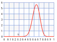
P(θ|z + α, N - z + β) = P(θ | 8 + 12.5, 2 + 12.5 ) = P(θ|20.5, 14.5)
- the Beta distribution graph would shift towards the right at this point and will have a higher density score because we added more trials.
- if our θ value for example, was 0.6, and your α and β at this point is 20.5 and 14.5, you should get a value of around ~4.7-4.8
- computing the formula is not required
Flip the coin ten more times (N) and observed 9 heads (z) out of 10.
α = 9
β = 1
P(θ|z + α, N - z + β) = P(θ| 9 + 20.5, 1 + 14.5) = P(θ|29.5, 15.5)
The graph keeps shifting to the right, so there is a probability that our coin is not 50/50 and therefore, not fair.
it becomes unlikely that the graph reaches a high point at the 0.5 mark.
In Bayesian Inference, the more data that becomes available, the more our beliefs get updated.
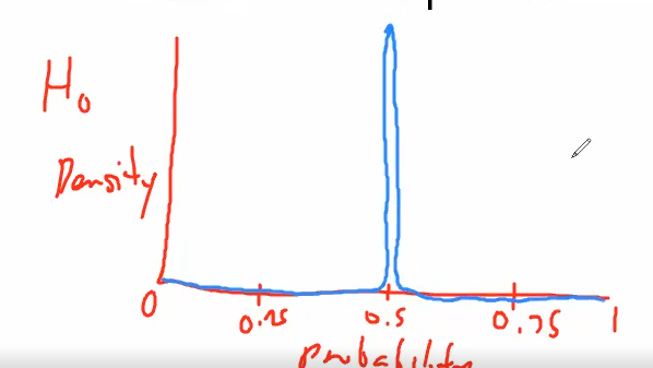
Hypothesis Testing
- Null Hypothesis: the infinity probability distribution only at a value of the parameter θ and zero probability elsewhere
- assume θ is 0.5
- the Beta distribution would look like this
- Alternative Hypothesis: all values of θ are possible, hence a flat curve representing the distribution
- the Beta distribution would look like this
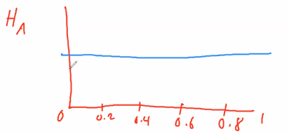
- the Beta distribution would look like this
Bayes Factors (equivalent of p-value)
- the Bayes Factor is the ratio between the posterior and prior odds
- where z is the number of successes
- N is the number of trials
- In practice, a value less than 0.1 is preferred to reject the null hypothesis H_0.
- in p-value, if value < 0.05, reject the null hypothesis
- in bf, if value < 0.1, reject the null hypothesis
the point of Bayesian Inference: Given new observations, how do we update our initial belief or initial assumption?
4a Association Rule Mining 🟢
Market-Basket Model
Frequent Itemset
Confidence
JcSites: Generating Association Rules
Market Basket Model
- this is used to describe a common form of many-to-many relationship between two kinds of objects
- Goal: identify items that are brought together by sufficiently many customers
- Approach: process the sales data collected with barcode scanners to find dependencies among items
- the barcode scanners record the transactions
Example
If a person buys cereal, we can reasonably assume that they're also buying milk. If a person buys coffee, they might buy sugar as well.
Assumptions about the data
- there is a large set of items
- there is a large set of baskets
- each basket contains a set of items (or itemset) - much smaller than the large set of all items
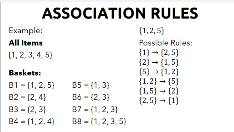
- Goal: discover association rules, which shows that people who bought the set {x, y, z} also tend to buy h
- given a large amount of transactions where each transaction contains at least one item (i.e. itemsets), we aim to discover rules which describe items that frequently appear in the same transactions
- association rules (or market basket analysis) are used to discover any interesting or meaningful relationships within the frequently grouped items
- so from the (list of transactions) → ((cereal → milk (90%), (bread → milk (40%)), (milk → cereal (23%)), (milk → apples (10%)))
Practical Applications of the Market Basket Model
- Store navigation
- Tie-in Promos
- Plagiarism Checker (ex. since 2022 when ChatGPT was released, the world "delve" was used a lot more in research papers)
- Side Effect Identification (ex. you give a set of medications to a patient, identify which guy has a certain side effect)
Frequent Itemset (definition of terms in Market Basket Model)
- let I = set of items
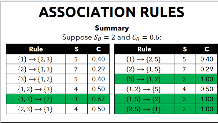
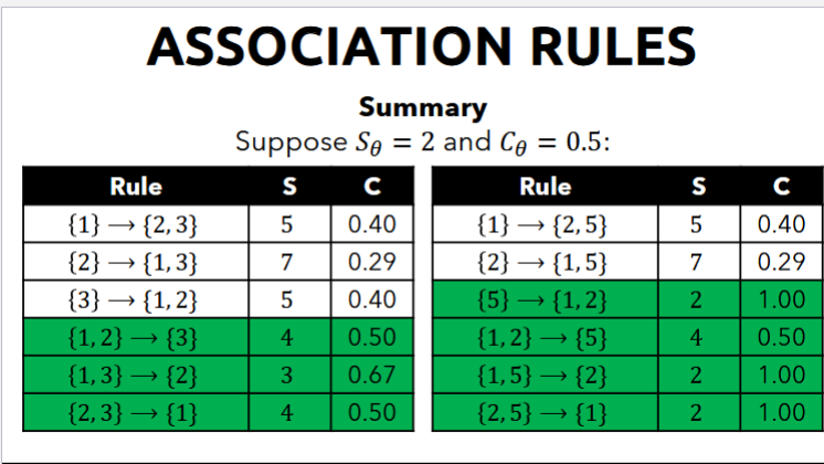
- let S_θ = a number called support threshold
- let S_I = the support of set I, which corresponds to the number of baskets for which I is a subset
- number of transactions that include that itemset I
- I is a frequent itemset if S_I ≥ S_θ
- an itemset with k items is referred to as a k-itemset
Example
All items I =
Baskets (we had 8 customers)
B1 = {milk, coke, beer}
B2 = {m, p, j}
B3 = {m, b}
B4 = {c, j}
B5 = {m, p, b}
B6 = {m, c, j, b}
B7 = {c, j, b}
B8 =
- Compute the Support S_I: how many people bought milk, coke, etc. these are 1-itemsets (k = 1)
S_{milk} = 5
S_{coke} = 5
S_{pepsi} = 2
S_{juice} = 4
S_{beer} = 6 - If our support threshold S_θ = 3...
S_{milk} = 5
S_{coke} = 5
S_{juice} = 4
S_{beer} = 6
are frequent itemsets - We look at the support of 2-itemsets where k=2... (pairs of items)
S{m, c} = 2
S_{m, j} = 2
S_{m, b} = 4
S_{c, j} = 3
S_{c, b} = 4
S_{j, b} = 2
S_{m, p} = 2
S_{c, p} = 0
S_{p, j} = 1
S_{p, b} = 1 - If our support threshold S_θ = 3...
S_{m, b} = 4
S_{c, j} = 3
S_{c, b} = 4
are frequent itemsets
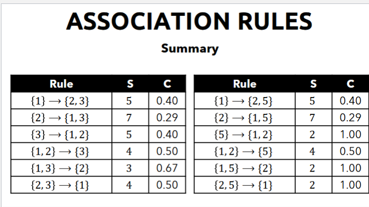
Confidence
- Confidence are if-then rules about the contents of baskets
- Rules are represented like this: {i_1, i_2, … i_k} → j means if a basket contains all i_1, i_2, …, i_k, then it is likely to contain j
- that's what we want to measure
- what's the probability that j will also be included given those items
- Confidence of association rules is the probability of j given
- probability of a customer buying item j given the items
- the Confidence C_{i_1, i_2, …, i_k} → j is the fraction of baskets with i_1, i_2, …, i_k that also contains j
Example
All items I =
Baskets (we had 8 customers)
B1 = {milk, coke, beer}
B2 = {m, p, j}
B3 = {m, b}
B4 = {c, j}
B5 = {m, p, b}
B6 = {m, c, j, b}
B7 = {c, j, b}
B8 =
We want to measure the confidence if someone buys {milk, beer} → coke
Confidence:
- where x = number of baskets with
- where y = number of baskets with
So the confidence of {milk, beer} → coke...
y = 4 (see highlighted)
x = 2
Example
We want to measure the confidence if someone buys {milk, beer} → pepsi
- x = number of baskets with {milk, beer, pepsi} = 1
- y = number of baskets with {milk, beer} = 4
Example
We want to measure the confidence if someone buys {milk, pepsi} → beer
- x = number of baskets with {m, p, b} = 1
- y = number of baskets with {m, p} = 2
Example
We want to measure the confidence if someone buys {coke, juice} → beer
- x = number of baskets with {c, j, b} = 2
- y = number of baskets with {c, j} = 3
Example
We want to measure the confidence if someone buys {coke, juice} → milk
- x = number of baskets with {c, j, m} = 1
- y = number of baskets with {c, j}= 3
When Association Rules are useful
Given an association rule {i_1, i_2, … i_k} → j, we can say that this association rule is useful iff:
- S_ {i_1, i_2, … i_k} ≥ S_θ: if the support for the set {i_1, i_2, … i_k} is greater than or equal to some support threshold S_θ
- C_{i_1, i_2, …, i_k} → j ≥ C_θ: if the confidence for the association rule {i_1, i_2, … i_k} → j is greater than or equal to some confidence threshold C_θ.
- confidence threshold is an arbitrarily assigned value
Example
All Items =
Baskets
B1 = {1, 2, 5}
B2 = {2, 4}
B3 = {2, 3}
B4 = {1, 2, 4}
B5 = {1, 3}
B6 = {2, 3}
B7 = {1, 2, 3}
B8 =
Compute the Support if S_θ = 2...
S_{1} = 5 (how many times does item 1 appear in a basket)
S_{2} = 7
S_{3} = 5
S_{4} = 2
S_{5} = 2
all of these are frequent item sets
Example
If we're looking for the frequent 2-itemsets and S_θ = 2...
S_{1, 2} = 4
S_{1, 3} = 3
S_{1, 4} = 1
S_{1, 5} = 2
S_{2, 3} = 4
S_{2, 4} = 2
S_{2, 5} = 2
S_{3, 4} = 0
S_{3 ,5} = 1
S_{4, 5} = 0
those that aren't highlighted are frequent 2-itemsets
Example
If we're looking for the frequent 3-itemsets and S_θ = 2...
S_{1, 2, 3} = 2
S{1, 2, 5} = 2
S_{1, 2, 4} = 1
S_{1, 3, 5} = 1
S_{2, 3, 4} = 0
S_{2, 3, 5} = 1
S_{2, 4, 5} = 0
those that aren't highlighted are frequent 3-itemsets
Note: if you increase the support of an itemset, the support will not increase.
Focusing on the 3-itemsets...
{1, 2, 3}
Possible Rules that we generated...
{1} → {2, 3}
{2} → {1, 3}
{3} → {1, 2}
{1, 2} → {3}
{1, 3} → {2}
{2, 3} → 1
We want to measure the confidence of these rules
Example {1} → {2, 3} if 1 is chosen, what's the probability that 2 and 3 will also be chosen
- x = number of baskets with
- y = number of baskets with
Example {2} →
Example {3} →
Example {1, 2} → {3} if 1 and 2 are chosen, what's the probability that 3 will also be chosen
- x = number of baskets with
- y = number of baskets with
Example {1, 3} →
Example {2, 3} →
If our confidence threshold was C_θ = 50%
{1} → {2, 3} = 0.40
{2} → {1, 3} = 0.29
{3} → {1, 2} = 0.40
{1, 2} → {3} = 0.50
{1, 3} → {2} = 0.67
{2, 3} → 1 = 0.50
only the highlighted will pass that threshold
Example with another set of rules: